

In naval architecture and marine engineering, open-water curves, such as the thrust, torque and efficiency are the primary hydrodynamic input to propeller and propulsion design. Capturing such quantities accurately through CFD modelling helps engineers take design decisions.
This article takes part of our ongoing HELYX Validation and Verification series, comparing the CFD results against the experimental data presented for the Potsdam Propeller Test Case (PPTC) case. As a secondary check, the same case was run with two different treatments of the interface between the rotating and stationary mesh regions, collocated cyclic AMI (Arbitrary Mesh Interface) and NCC (Non-Conformal Coupling), to compare the accuracy and computational cost of both approaches.

The Potsdam Propeller Test Case (PPTC) Benchmark
The PPTC is built around model propeller VP1304, a five-bladed propeller of diameter D = 0.25 m, measured in open water conditions at SVA Potsdam [1]. It is a widely used validation benchmark because both the geometry and the measured open-water data are public, and because it was the subject of the SMP’11 workshop [2], which produced a body of published solver-to-solver comparisons.
For this study the propeller runs at a constant 900 RPM and the operating point is varied through the inflow velocity, matching the experimental procedure. Performance was evaluated at 11 different values of advance coefficient.
The compared quantities are the standard open-water characteristics:
- Advance coefficient: J = V∞ / (N·D)
- Thrust coefficient: KT = T / (ρ·N²·D⁴)
- Torque coefficient: 10·KQ = 10·Q / (ρ·N²·D⁵)
- Open-water efficiency: η = J·KT / (2π · 10·KQ/10)
Where V∞ is the advance speed, N the propeller speed, D the propeller diameter, T the thrust, Q the torque and ρ the fluid density. Thrust and torque are sampled with the forces function object on the rotating sections of the propeller blades.
With N and D fixed, J is set entirely by the inflow advance speed: V∞ = 3.75·J m/s. The tested range of roughly J = 0.47 to J = 1.58 therefore corresponds to inlet velocities of about 1.8 m/s to 5.9 m/s, while the blade tip speed stays constant at π·N·D ≈ 11.8 m/s. Because η is a ratio of KT to KQ, errors in the predicted forces propagate directly into the efficiency curve.
Configuring the Marine Propeller CFD Simulation in HELYX
The case is modelled as steady-state, isothermal and incompressible, using the HELYX incompressible solver with the k-ω SST turbulence model and wall functions. The propeller blades are defined as stationary in a rotating reference frame specified at the rotation speed.
The far-field domain is 2.56 m long (10.2 D) with a 0.6 m × 0.6 m cross-section (2.4 D per side), with the propeller shaft entering from the upstream face. The inlet is a velocity boundary condition — this is what sets the advance coefficient for each of the 11 runs — the outlet is a pressure boundary condition, and the domain walls are no-slip.

Setup at a glance
| Parameter | Value |
| Propeller model | VP1304, five-bladed, D = 0.25 m |
| Rotational speed | 900 RPM, constant |
| Operating points | 11 advance speeds (J ≈ 0.47–1.58) |
| Far-field domain | 2.56 m long, 0.6 m × 0.6 m cross-section |
| Outlet | Pressure |
| Domain walls | No-slip |
| MRF zone | Cylinder, 0.3 m diameter × 0.18 m long |
| Rotating-zone | interface Collocated cyclic AMI / NCC |
| Mesh | 1.84 M cells (far-field + propeller region, merged) |
| Physics | Steady-state, incompressible, isothermal |
| Turbulence model | k-ω SST with wall functions |
| Computational settings | 32 processes, cluster of AMD EPYC 7251 8-core nodes, 128 GB RAM per node |
Mesh Strategy and Case Setup
Mesh quality and cell count drive both accuracy and computational cost. Rather than generating a single grid for the whole domain, the far-field domain was discretised and meshed separately from the propeller and its MRF zone, and the two grids were then merged into the final mesh of 1.84 million cells.
The advantage is that refinement is decided per region: the propeller region is sized to resolve the blade surfaces and hub, while the far field is meshed only as finely as the far-field flow requires. It also lets the propeller mesh be regenerated or re-refined without rebuilding the far field. The consequence is a non-conformal boundary between the two regions, which has to be handled by an interface treatment — discussed below.
Rotation is modelled with the Multiple Reference Frame (MRF) method: inside the marked cell zone the equations are solved in a frame rotating at the propeller’s angular velocity, the mesh itself does not move, and the blades stay frozen in position relative to the surrounding domain. The MRF zone here is a cylinder of 0.3 m diameter (1.2 D) and 0.18 m axial length around the propeller.
For open-water conditions this is not a crude approximation. The inflow is uniform and axial and the surrounding domain is axisymmetric, so the flow really is steady in the blade-fixed frame and MRF resolves it at a fraction of the cost of a transient run. MRF stops being appropriate when the inflow seen by the blades varies with angular position — behind a hull, in oblique flow — or when blade-passing loads, unsteady cavitation or hull-pressure pulses are the quantity of interest. Those require a transient sliding-mesh solution. The same reasoning governs rotating machinery generally; see our NASA Rotor 67 turbomachinery validation.


Two Interface Treatments for the Rotating Region
Because the far-field and propeller meshes are generated separately, their faces do not match one-to-one where the two regions meet. HELYX offers two treatments for that boundary, and the case was run with each:
- AMI (Arbitrary Mesh Interface): the
AMIboundary type creates a fully coupled interface from a pair of patches that share the same geometrical shape but may carry different numbers of faces. Fields are transferred between the two patches by interpolation across the pair. - NCC (Non-Conformal Coupling): with the NCC boundary type the two original patches remain uncoupled, and the coupling is instead constructed on demand as additional generated patch pairs which are populated with faces in the finite-volume mesh. NCC was designed to produce more conservative results in coupled mesh regions than the standard AMI coupling. It is a more recent addition to HELYX, and reducing its computational cost is an area of ongoing development.
The relevant question for this validation is not which is cheaper, but whether the choice perturbs the predicted forces. Running the identical mesh, physics and operating points through both isolates that effect.
Results: CFD vs. Experimental Data
The propeller’s performance was evaluated at 11 different advance coefficients, corresponding to varying inlet velocities. The non-dimensional performance metrics — Thrust Coefficient (KT), Torque Coefficient (10KQ), and Efficiency (η)—were calculated from the forces and moments acting on the propeller blades.
The HELYX simulation results show excellent agreement with the experimental data from SVA Potsdam across the entire operating range. The plots below illustrate a tight correlation for both thrust and torque coefficients, which translates directly into an accurate prediction of overall propeller efficiency.
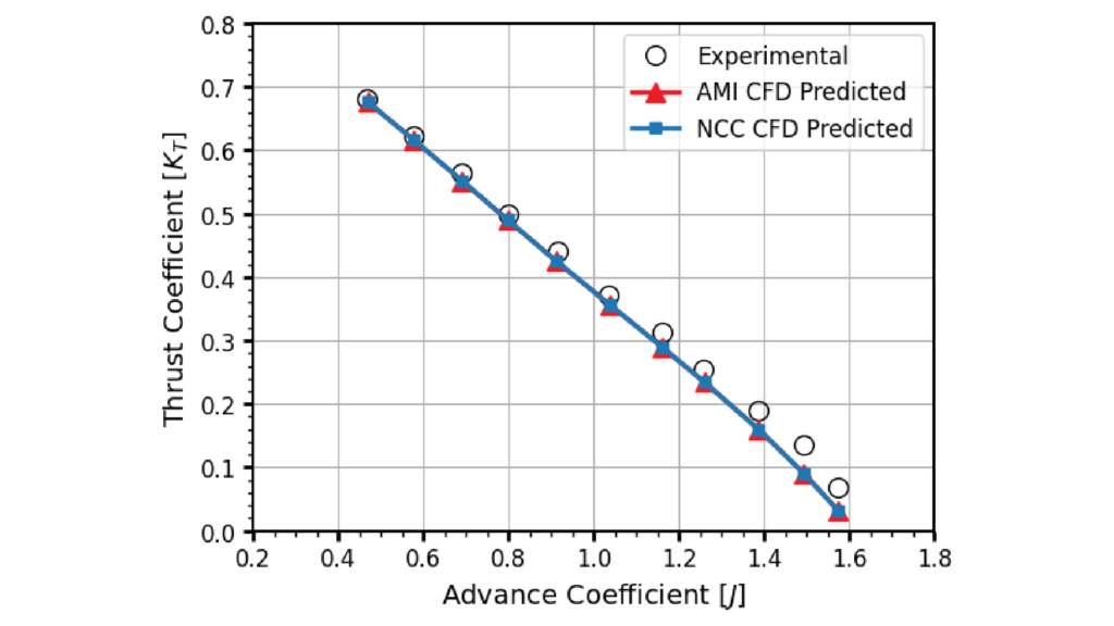
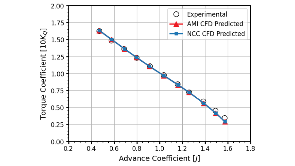
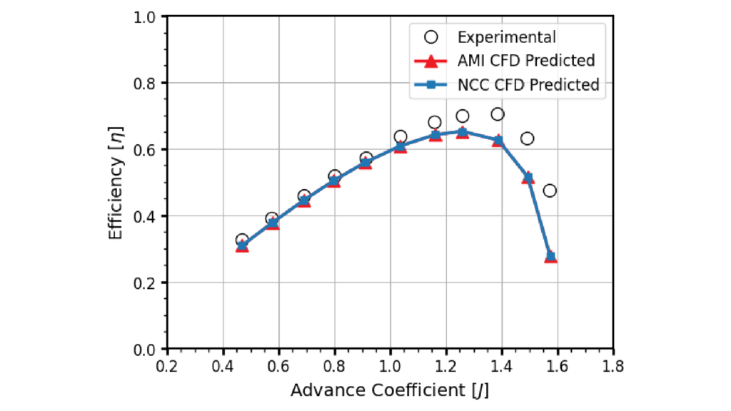
Agreement in KT and KQ is close from the lowest J up to approximately J = 1.2, which covers the loaded and design-range operating points. At higher J the predicted thrust falls below the measured values, and the efficiency curve inherits and amplifies that deviation. This is expected rather than anomalous: as the propeller unloads towards zero thrust, KT becomes small, so a fixed absolute error becomes a large relative error, and efficiently carries it through directly. Confidence in these results is therefore highest through the loaded range and around the efficiency peak, and lowest in the lightly loaded tail.
The AMI and NCC curves are effectively superimposed across the whole range. Quantitatively:
| Coupling type | RMSE KT (%) | RMSE KQ (%) | Run time |
|---|---|---|---|
| AMI | 2.3090 | 2.0514 | 4h 40m 59.8s |
| NCC | 2.3069 | 2.0504 | 7h 01m 13.8s |
- RMSE for Thrust Coefficient (KT): ~2.3%
- RMSE for Torque Coefficient (KQ): ~2.05%
The two treatments differ by 0.002 percentage points in KT and 0.001 in KQ — three orders of magnitude below the ~2% deviation from experiment, and effectively at the level of solver convergence noise. For this case the interface treatment is not a source of error in the predicted loads; the residual discrepancy against the measurements comes from elsewhere in the model.
Run times are reported for completeness. Both runs used 32 processes on a cluster of AMD EPYC 7251 8-core nodes with 128 GB RAM per node.
Conclusion: Achieve Accurate Results 33% Faster with HELYX
HELYX reproduces the PPTC open-water curves with RMSE of 2.31% on KT and 2.05% on KQ across 11 advance coefficients, using a steady-state MRF model on a 1.84 million cell mesh running on 32 cores. Errors of this order in both thrust and torque are within the band normally required for open-water performance prediction and for ranking design variants in a parametric study.
The result is insensitive to how the rotating and stationary mesh regions are coupled: AMI and NCC return the same coefficients to three significant figures. That matters for anyone building a propeller workflow in HELYX, because it means the interface treatment can be chosen on other grounds — mesh topology, or the improved conservation NCC is designed to deliver — without revalidating the loads.
To discuss how HELYX fits your marine and rotating machinery workflows, contact our team for a consultation.
References
[1] U. Barkmann. Potsdam Propeller Test Case (PPTC) – Open Water Tests with the Model Propeller VP1304. Tech. rep., Schiffbau-Versuchsanstalt Potsdam, 2011.
[2] L. Lübke. Potsdam SMP’11 Workshop. Schiffbau-Versuchsanstalt Potsdam, 2011. https://www.sva-potsdam.de/en/pptc-smp11-workshop