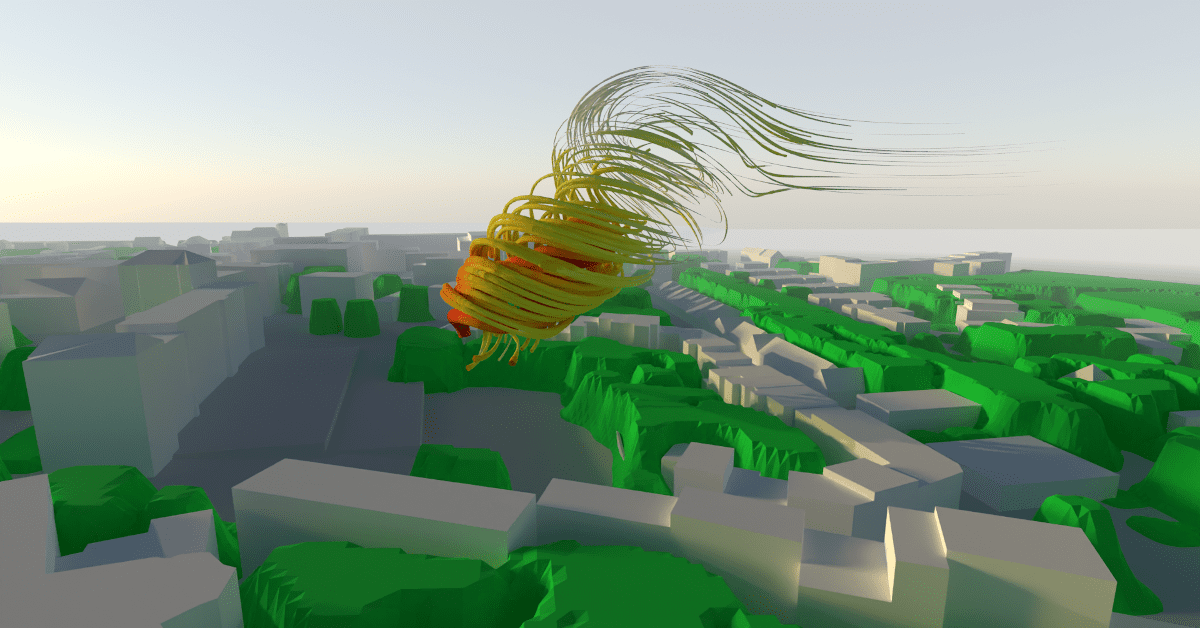
In central Europe, in the height of summer, especially in the evening of hot days, it is not uncommon to experience heavy thunderstorms. During one such event in summer 2019, I witnessed, what looked like, a dust devil forming for a few moments, which then also ripped off the larger part of the roof of the house I live in.
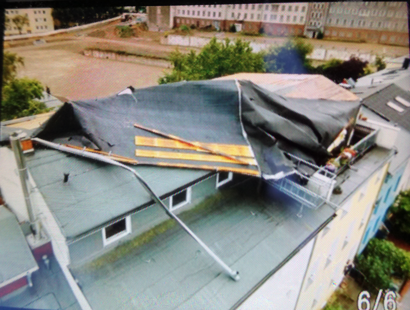
After the worst of the damage had been fixed, the idea formed to go after the event with CFD simulations. Or at least attempt to do so, realizing that I would face a long list of unknown or uncertain boundary and initial conditions.
Initial Considerations – Location
In the photo one can see the view I had, being outside at this time, trying to secure the laundry from approaching dark clouds. (The photo was taken a few days later.)
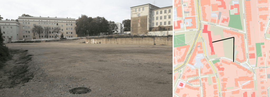
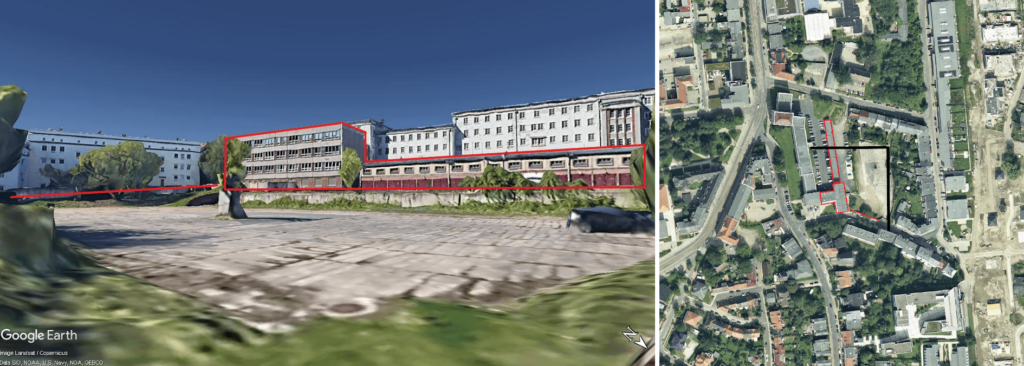
A recent demolition of a building (more on this later) and reworking of the area by the city council resulted in a large flat area, covered by sand and dirt. The building in the back (right) plays a major role in the unfolding events. At least that’s what I suspected, going into this little project.
Here is roughly the same view from Google Earth still showing the demolished building and structures.
Initial Considerations – Conditions
First off, I should qualify, that I did not witness a tornado or dust devil, which form in different ways involving thermal gradients and Coriolis forces. This is not what happened here. I suspected that a strong squall of wind created a separation on the larger building’s edge. This vortex was quite large, though, with roughly 50m diameter and reaching up maybe 50m or more. It was made visible by all the dust and sand in that area being sucked up and lasted for around 5 seconds. That would be my eye-witness statement. What made this so extraordinary was certainly the sudden onset of the squall and forming of the vortex and of course the fact that seconds later my roof was gone.
So, what were the conditions. Usually, we get winds from the WSW and later searching the weather records confirmed the thunderstorm front approaching pretty much from the west. Furthermore, the weather services issued a warning for that evening with squalls reaching up to 110km/h (Bft 11).
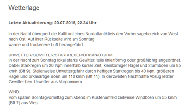
From later searching the actual records from nearby stations, the peak wind speed was indeed up to 110km/h that evening. Again, the sudden onset was noticeable, with the weather being very calm before. Since I suspected this to be a phenomenon of a separation from a large building, I ignored any thermal or humidity conditions.
So, I am looking at a quickly ramping up wind profile hitting the area from 270°. That should be fine to feed into the CFD model.
Building the Model
Onwards to creating the CAD model. I am looking for a realistic representation of the buildings in a certain radius around the vortex area. The OpenStreetMap project provides this kind of data. Back in 2019 when I first worked on this, I used a rather involved process, which I still want to mention here, to give credit to the tool I used back then. The process included exporting the map data from OpenStreetMap.org and feeding it into a little program called OSM2World which creates a 3D representation of the map. This can then be exported out of OSM2World as an *.obj file. That *.obj file than gets imported into Blender. The data did not include any 3D information on the terrain, so that needed to be done manually as well, basically creating the underlying height map of the area and projecting the buildings onto it. There is a slight 15m slope in the area, which might be of importance. Otherwise, the area is pretty flat.
More recently, I stumbled upon a Blender Add-On, that does all that in one step, BlenderGIS, which is free to use. There is an excellent YouTube video about how to use it, which is basically what I followed.
Both methods rely on OSM data and need some clean-up / correction to make it more accurate, at least close to the area of interest. This includes height of buildings and shape of roofs.
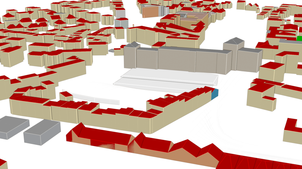
Just west of the area of interest lies a park that stretches in W-E direction and which comes in as either a collection of primitive tree models using the first process or empty space using BlenderGIS. I suspected the presence of the trees in that park as well as in other locations might have an impact on the results, so I planned to rely on the vegetation modelling functions coming with HELYX. Basically, the vegetation is assigned a cell zone or volume inside the computational mesh and the model accounts for momentum, thermal and humidity influences due to the vegetation density in those zones.
But how to get the vegetation volume. I used publicly available infrared satellite pictures of the area, in which vegetation can be detected.
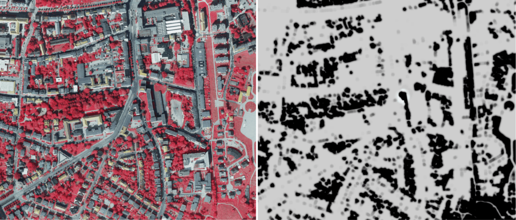
Based on that picture it is possible to create a mask or height map in Blender and use it to “grow” a vegetation volume. Since grass comes up as red as well in the satellite picture, I ended up with rather more trees than are present in reality, so a bit of manual clean-up was again necessary near the area of interest.
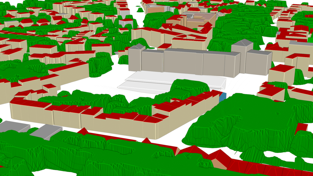
All that’s left now is to define the outer bounds of the model. Choosing a cylindrical farfield (diameter of ~1500m, height ~500m ) in case I want to play around with the wind direction.
Simulation Setup
Using HELYX’s dual mesher to ensure 100% near wall layer coverage on the buildings, I arrive at a 10 million cell mesh after placing refinement volumes in the area of interest. Cells that fall within the vegetation are automatically assigned to a single cellZone. And that already concludes the meshing stage. Since the HELYX mesher can handle dirty CAD just fine, there was no need to fix any geometry. In fact, the ground, the vegetation and the buildings are intersecting each other all over the place, but posing no problems for the mesher.
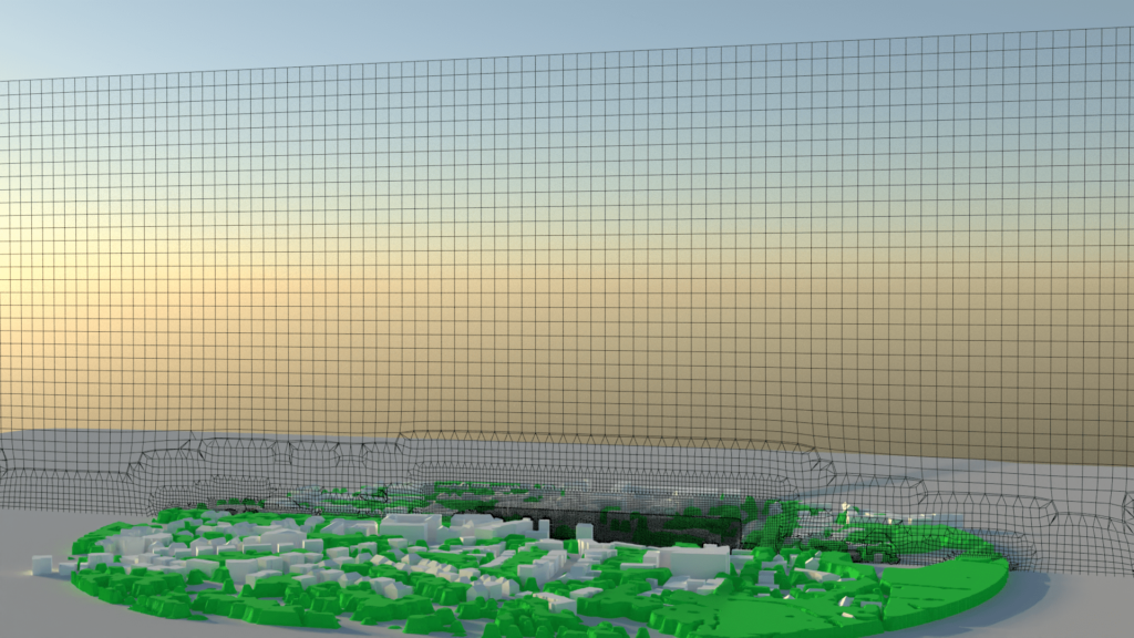
Onwards to the flow setup. Obviously, this will be a transient simulation. Using the wind profile boundary condition on the cylindrical boundary, I define a simple boundary layer profile which ramps up in time from 0 to full speed after 5 seconds coming from the west. That should be sufficient to represent the squall.
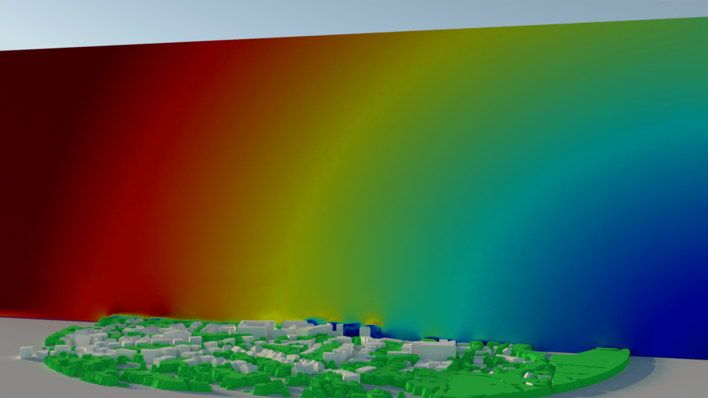
The vegetation zone gets set up using the simplest of the options HELYX offers, using a uniform leaf area density (LAD) profile to affect the porosity inside the cellZone.
Running for 30s should be sufficient for the squall front to run over the area of interest. Based on the cell size and expected velocities I chose a constant time step of dt=0.01s.
And then all that is left, is waiting for a free slot on the cluster to run this little pet project. In the end the run took less than 5 hours on 128 cores.
Results
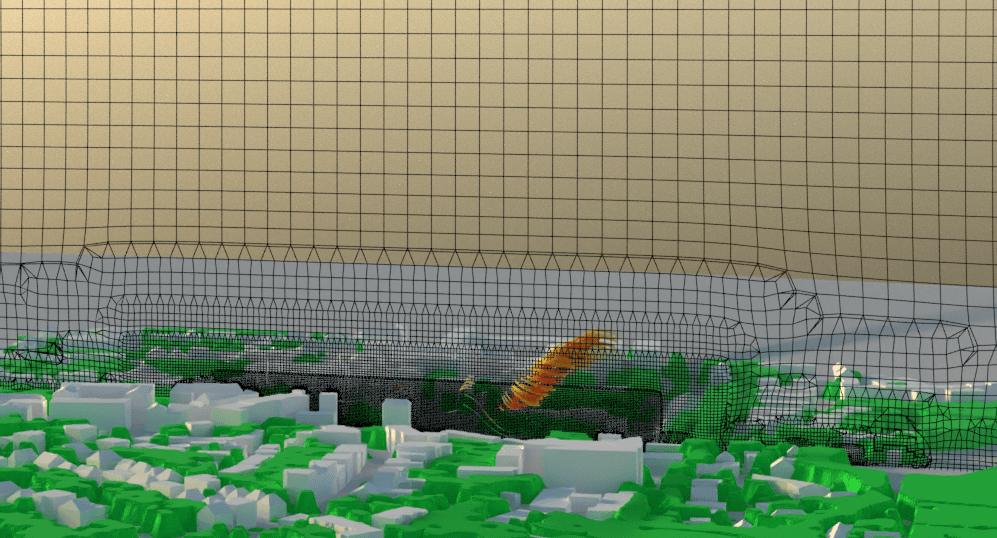
I was frankly amazed that I caught the vortex in the first attempt. Considering how much guessing went into the preparation and the setup of the model I was either very lucky to have met the correct conditions or the forming of the vortex is so common that it happens all the time. Speaking against that latter, is the fact that in real life I only witnessed it once. The location of the vortex is spot on and the duration between it forming and the eventual dissolving also matches what I witnessed. What was surprising was the vertical extent of the vortex. Easily more than twice as high as tallest buildings in the vicinity. Here is a comparison against the local mesh size. Any re-runs would need the local mesh refinement to extend further in vertical direction.
Given the limited time and resources available for this project and being quite happy that the first run seems to have used pretty accurate conditions, there is one particular comparison simulation I wanted to make. As mentioned in the beginning, the city council demolished a house near the area where the vortex formed just days before the event. I was curious to see whether the absence of that building was responsible in any way.
Plugging the missing building into the CAD and resurrecting a couple of felled trees and walls (who knows?!) was easy and a second run was started.
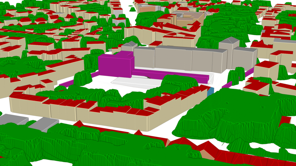
Nothing interesting to show in terms of results. The squall passes over the area, some chaotic separations, no lasting coherent flow structures whatsoever form!
Conclusions
It was an interesting journey to go through the whole process of creating a wind simulation for a city using a number of tools and resources to arrive at a solution that was experienced first-hand. Being able to show that, as suspected, the absence of the demolished building had directly led to the forming of the vortex with comparatively little effort was amazing. CAD model generation and final polished animation was done with Blender, which is just perfect for the job. Doing the meshing, setup and running in HELYX was also straightforward.
Addressing the actual damage to my roof. Seeing an indication of this in the simulation would have been asking for too much, I think. The level of detail of the buildings was not high enough to accurately represent roof forms and structures below 1m. Same goes for the mesh resolution. On top of that it is not necessarily given that the vortex had anything to do with a local low pressure spike on a nearby roof.
In terms of potential future work, one could easily combine the Python based journaling of the HELYX setup process to automatically run through a matrix of different wind directions and speeds. That would show how sensitive the vortex really is to those parameters. Combining this with automatic monitoring the swirl in the area of interest, one could even forego any time consuming postprocessing whilst running through the matrix.
All in all a fun little project, that I am happy to be able to share.

